Methods using individual frequencies
Using grids that include theoretically computed oscillation frequencies (see Grids of models) BASTA can fit these
individual frequencies with a surface correction, as well as combination of frequencies. In the following we show
examples of the blocks that must be modified in create_inputfile.define_input() to produce these types of fits.
Individual frequencies: main sequence
BASTA is shipped with individual frequencies for the Kepler main-sequence target 16 Cyg A derived by
Davies et al. 2015. These are included in the
ascii file BASTA/examples/data/freqs/16CygA.fre and listed in columns of
(order, degree, frequency, error, flag). To fit these frequencies to a grid of models, the ascii input must be converted
to a suitable xml file with the routine fileio.freqs_ascii_to_xml(). Simply run the following commands in
the terminal:
cd BASTA
source venv/bin/activate
cd examples/data/freqs
python3
from basta import fileio; fileio.freqs_ascii_to_xml('.', '16CygA')
Which gives the output:
Star 16CygA has an epsilon of: 0.8.
No correction made.
This will produce the file 16CygA.xml, which can be used as a direct input in the BASTA fitting.
The ascii file must a header naming the different columns and at a minimum the file must contain:
the mode frequencies in µHz, typically named freq or frequency in header
the angular degrees l, typically named l, ell or degree
- the uncertainties of the mode frequenciea in µHz. These can either be
symmetrical and thus only a single column with an uncertainty can be given, typically denoted error or err.
asymmetrical. In this case, the upper and lower uncertainty must be given as two separate columns, typically denoted error_plus and error_minus.
Furthermore, feel free to add a column containing radial orders (order or n) if these are known.
For convenience, you can check your column of radial orders based on the calculated epsilon value.
This is done by including an additional argument in the python command:
from basta import fileio; fileio.freqs_ascii_to_xml('.', '16CygA', check_radial_orders=True)
This will then output:
Star 16CygA has an epsilon of: 0.8.
The proposed correction has been implemented.
BASTA calculates the epsilon (\(\epsilon\)) term as described in White et al. 2012 and correct the radial order of the frequencies accordingly. In this case the radial order of the input frequencies is already appropriate, and thus BASTA does not change the values of the radial order.
With the input file in the appropriate xml format, the following blocks must be modified in create_inputfile.py:
# ==================================================================================
# BLOCK 2: Fitting control
# ==================================================================================
define_fit["fitparams"] = ("Teff", "FeH", "freqs")

# ------------------------------------------------------------
# BLOCK 2d: Fitting control, frequencies
# ------------------------------------------------------------
define_fit["freqparams"] = {
    "freqpath": "BASTA/examples/data/freqs",
    "fcor": "BG14",
    "correlations": False,
    "dnufrac": 0.15,
}

# ==================================================================================
# BLOCK 4: Plotting control
# ==================================================================================
define_plots["freqplots"] = "echelle"
This defines freqs as a fitparam in block 2. Block 2d gives the path to the frequency xml-file, sets the
frequency correction from Ball & Gizon 2014,
ignores correlations between individual frequencies, and restricts the lowest l=0 mode from each model to be within 15%
of the value of the observed one.
We have provided an ready-to-run example for this star:
cd BASTA
source venv/bin/activate
cd examples/xmlinput
python create_inputfile_freqs.py
BASTArun input_freqs.xml
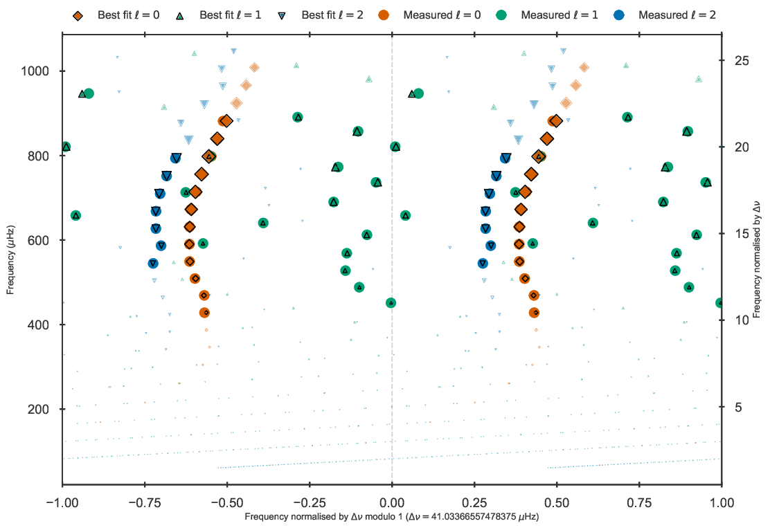
The fit should take less than a minute and the output is stored in BASTA/examples/output/freqs. Besides the
corner plot and Kiel diagrams, the code produces output of the fit to the individual frequencies in form of echelle
diagrams for both corrected and uncorrected frequencies:
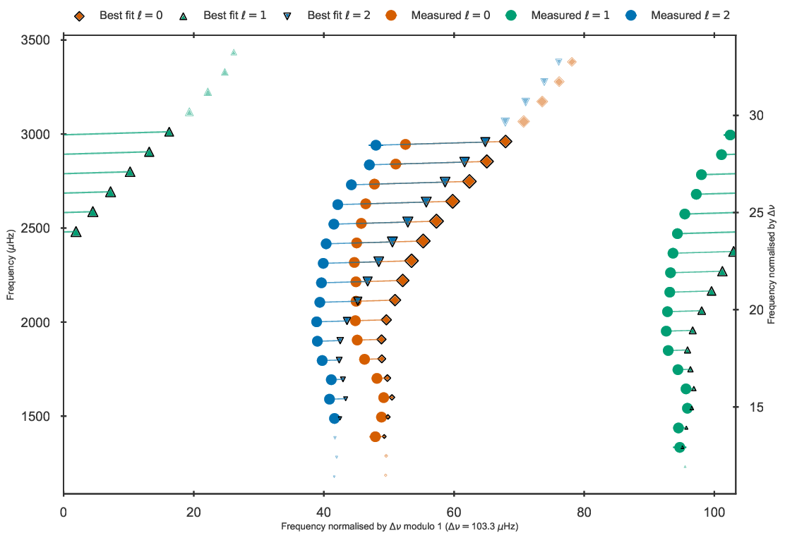
Echelle diagram showing the uncorrected frequencies of the best fit model to 16 Cyg A in the grid.
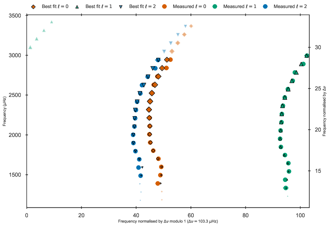
Echelle diagram after the BG14 frequency correction to the best fit model to 16 Cyg A in the grid.
Frequency ratios
BASTA also has the option to fit the frequency ratios (\(r_{01}, r_{10}, r_{02}, r_{010}, r_{012}\)). To do this,
one simply adds the following fitparam (for the case of \(r_{012}\) as an example):
# ==================================================================================
# BLOCK 2: Fitting control
# ==================================================================================
define_fit["fitparams"] = ("Teff", "FeH", "r012")

# ==================================================================================
# BLOCK 4: Plotting control
# ==================================================================================
define_plots["freqplots"] = "ratios"
The variable freqplots can also be set to True, which will produce plots of the ratios and corresponding echelle
diagrams even though individual frequencies are not fitted. We provide an example to run this fit in
BASTA/examples/xmlinput/create_inputfile_ratios.py which produces the file input_ratios.xml. Running
this file stores the results of the fit in BASTA/examples/output/ratios/, and the resulting ratios should look
as follows:
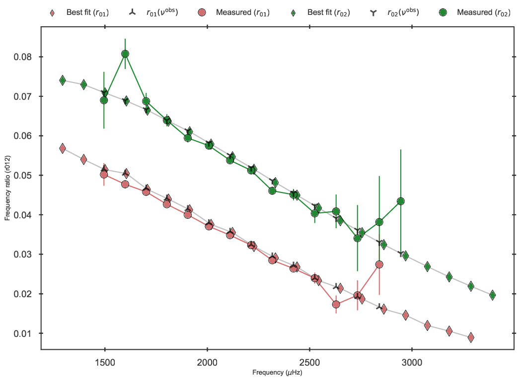
Frequency ratios of the best fit model to 16 Cyg A in the grid.
BASTA uses by default the five-point small frequency separation formulation for computing the ratios, which is the recommended option. Additionally, interpolation of the model ratios to the observed frequencies are applied in the fit. Finally, the correlations between the ratios are taken into account by using the full covariance matrix. Any of these settings can of cource be changed should the user wish to do so.
Epsilon differences
Similar to frequency ratios, BASTA can also fit the surface-independent frequency phase differences, commonly
referred to as epsilon differences (Winther et. al, in preparation). The individual set of differences
(\(\delta\epsilon_{01}, \delta\epsilon_{02}\)) as well as the combined set can be fitted by adding the
correpsonding keyword to fitparams (here for the case \(\delta\epsilon_{012}\)):
# ==================================================================================
# BLOCK 2: Fitting control
# ==================================================================================
define_fit["fitparams"] = ("Teff", "FeH", "e012")

# ==================================================================================
# BLOCK 4: Plotting control
# ==================================================================================
define_plots["freqplots"] = "epsdiff"
Adding epsdiff to freqplots produces the corresponding figure, which can also generally be produced when
individual frequencies are available. An example of how to run this fit is provided in
BASTA/examples/xmlinput/create_inputfile_epsilondifference.py which produces the file input_epsilondifference.xml.
Running this file stores the results of the fit in BASTA/examples/output/epsilon/, and the resulting
epsilon differences should look as follows:
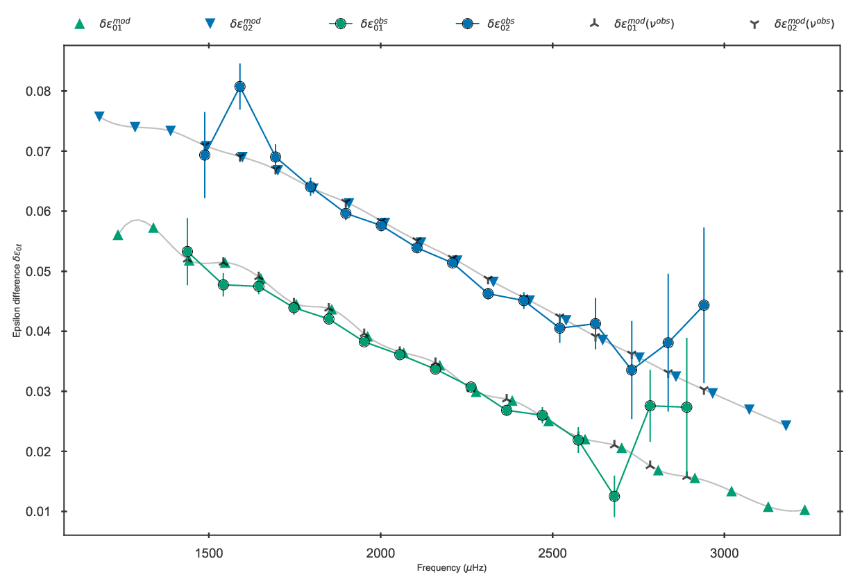
Epsilon differences of the best fit model to 16 Cyg A in the grid.
Note that since the determination of epsilon differences relies on interpolating the \(\ell=0\) epsilons to the frequency locations of the \(\ell=1,2\) modes, one would extrapolate the \(\ell=0\) epsilons if the frequency locations of the \(\ell=1,2\) goes outside the interval of the frequency locations of the \(\ell=0\) modes. These are therefore excluded, and thus the number of epsilon differences may not be equal to the number of \(\ell=1,2\) frequencies.
As noted above for the ratios, correlations/covariances are taken into account in the fit.
Frequency glitches
Important: To use this feature, please compile the required modules! Please refer to the installation instructions for help.
Another feature of BASTA is the fit of frequency glitches related to the He ionisation zones. These are comprised of three parameters, which are:
the average amplitude of the He glitch signature, \(\langle A_{He}\rangle\,(\mu Hz)\),
the acoustic width of the He glitch signature, \(\Delta_{He}\,(s)\),
and the acoustic depth of the He glitch signature, \(\tau_{He}\,(s)\).
These can be precomputed and provided by the user in hdf5 format, by either computing them using the
GlitchPy code, or following the file structure defined within.
If not precomputed, these can be computed from the provided individual frequencies. In this case, the method used in GlitchPy is adapted, whereby the method by which the glitch parameters are determined needs to be defined in block 2f as e.g.
# ------------------------------------------------------------
# BLOCK 2f: Fitting control, glitches
# ------------------------------------------------------------
define_fit["glitchparams"] = {
    "method": "Freq",
    "npoly_params": 5,
    "nderiv": 3,
    "tol_grad": 1e-3,
    "regu_param": 7,
    "nguesses": 200,
}
The number of realisations to use in the MC scheme to derive the observed glitch parameters are set by the nrealizations keyword
in the freqparams dictionary (block 2d).
If the glitch parameters are provided in the GlitchPy format, the method by which these were computed will instead be adopted. The file
must be provided as *star_id*.hdf5, in the same directory as the individual frequencies. The readglitchfile keyword in the
freqparams dictionary (block 2d) can then be set to True to allow the precomputed glitches to be read.
To produce the fit one simply needs to include the appropriate parameter glitches in fitparams
# ==================================================================================
# BLOCK 2: Fitting control
# ==================================================================================
define_fit["fitparams"] = ("Teff", "FeH", "glitches")
The option to fit glitches together with frequency ratios is also provided, whereby the correlations between
the ratios and glitch parameters of the observations are derived and applied. This option is simply enabled by relacing glitches in
fitparams by the desired frequency ratio sequence preceded by a g, as e.g. gr012 for fitting glitches along with the r012
sequence.
You can find the corresponding python script to produce the input file for this fit in
BASTA/examples/xmlinput/create_inputfile_glitches.py. Running this example produces output located in BASTA/examples/glitches/,
where the fitted glitch parameters are shown in 16CygA_gltches_gr012.png, which should look as follows:
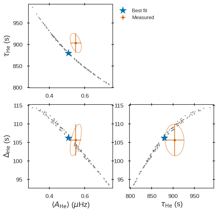
Fitted glitch parameters of 16 Cyg A fitted using glitches and ratios.
Individual frequencies: subgiants
Reproducing the frequency spectrum of subgiant stars is a challenging task from a technical point of view, as the radial order of the observed mixed-modes does not correspond to the theoretical values used to label them in models. We have developed an algorithm that deals with this automatically, and we refer to section 4.1.5 of The BASTA paper II for further details.
In practice, you simply need to provide an ascii file with the individual frequencies in the same format as in the
main-sequence case (order, degree, frequency, error, flag). The radial order given is basically irrelevant, as BASTA
will use the epsilon (\(\epsilon\)) method to correct the radial order of the l=0 modes, and use only the frequency
values for the l=1,2 modes to find the correct match.
We include an example of frequencies for a subgiant in the file BASTA/examples/data/freqs/Valid_245.fre. It
corresponds to one of the artificial stars used for the validation of the code as described in section 6 of
The BASTA paper II. Quick exploration of the file
reveals that it has a number of mixed-modes of l=1 that have radial orders labelled in ascending order. You need to
transform the .fre file into a .xml file following the usual procedure:
cd BASTA
source venv/bin/activate
cd examples/data/freqs
python
from basta import fileio
fileio.freqs_ascii_to_xml('.','Valid_245',check_radial_orders=True,nbeforel=True)
You should see the following output:
Star Valid_245 has an odd epsilon value of 1.9,
Correction of n-order by 1 gives epsilon value of 0.9.
The proposed correction has been implemented.
The input is now ready. The global parameters of the star are contained in BASTA/examples/data/subgiant.ascii.
To run the example, a few modifications to create_inputfile.define_input() are necessary (related to input
files and grid to be used). The following blocks are now changed:
# ==================================================================================
# BLOCK 1: I/O
# ==================================================================================
xmlfilename = "input_subgiant.xml"

define_io["gridfile"] = "BASTA/grids/Garstec_validation.hdf5"

define_io["asciifile"] = "BASTA/examples/data/subgiant.ascii"
define_io["params"] = (
    "starid",
    "Teff",
    "Teff_err",
    "FeH",
    "FeH_err",
    "dnu",
    "dnu_err",
    "numax",
    "numax_err",
)
A ready-to-run file is provided in BASTA/examples/xmlinput/create_inputfile_subgiant.py and as usual it can
simply be run as
cd BASTA
source venv/bin/activate
cd examples/xmlinput
python create_inputfile_subgiant.py
BASTArun input_subgiant.xml
The resulting duplicated echelle diagram should look as like the following.
Echelle diagram after the BG14 frequency correction to the best fit model to Validation star 245.
The corner plot present peaks revealing the underlying sampling in the code. Once again we refer you to the section on Interpolation of tracks and isochrones to refine the grid as desired.