Isochrones, distances, and evolutionary phase
BASTA is shipped with a complete set of isochrones from the BaSTI library. The input physics, science cases, and mixtures are described in the Solar scaled paper and the Alpha-enhanced paper. We show here how these isochrones can be used to determine stellar properties while fitting asteroseismic data, parallaxes, and a prior on the evolutionary phase of a star.
In BASTA/examples/data/ we have included the file Kepler_RGB.ascii, which contains the global parameters
of the red giant branch star KIC 11129442 observed by the Kepler satellite. Besides spectroscopic properties and
asteroseismic observables, the file contains magnitudes in the 2MASS system, parallax from Gaia eDR3, and evolutionary
phase as determined from its asteroseismic period spacing. Necessary changes to create_inputfile.define_input()
are the following:
# ==================================================================================
# BLOCK 1: I/O
# ==================================================================================
define_io["gridfile"] = "grids/BaSTI_iso2018.hdf5"

define_io["asciifile"] = "data/Kepler_RGB.ascii"
define_io["params"] = (
    "starid",
    "RA",
    "DEC",
    "Teff",
    "Teff_err",
    "FeH",
    "FeH_err",
    "dnu",
    "dnu_err",
    "numax",
    "numax_err",
    "Mj_2MASS",
    "Mj_2MASS_err",
    "Mh_2MASS",
    "Mh_2MASS_err",
    "Mk_2MASS",
    "Mk_2MASS_err",
    "parallax",
    "parallax_err",
    "phase",
)
Which reads the variables from the input file. To work with the isochrones, block 2c needs to be used for defining the desired science case:
# ------------------------------------------------------------
# BLOCK 2c: Fitting control, isochrones
# ------------------------------------------------------------
define_fit["odea"] = (0.2, 0, 0.3, 0)    # + mass loss
This will select the isochrones including overshoot in the main sequence, no microscopic diffusion, with mass-loss, and no alpha-enhancement.
Fitting parallax
The first fit in this example will include spectroscopy, global asteroseismic parameters, and parallax. The
fitparams entry must be modified:
# ==================================================================================
# BLOCK 2: Fitting control
# ==================================================================================
define_fit["fitparams"] = ("Teff", "FeH", "dnuSer", "numax", "parallax")
Note that we fit the large frequency separation using the
Serenelli et al. 2017 correction (called dnuSer)
instead of dnufit since theoretical oscillation frequencies are not included in isochrones (see section 4.1.1 of
The BASTA paper II). In order to fit the parallax,
we need to provide at least one apparent magnitude. This is done modifying block 2e as follows:
# ------------------------------------------------------------
# BLOCK 2e: Fitting control, distances
# ------------------------------------------------------------

define_fit["filters"] = ("Mj_2MASS", "Mh_2MASS", "Mk_2MASS")

define_fit["dustframe"] = "icrs"
We will use all 3 apparent magnitudes from 2MASS and we specify the reference frame for the input coordinates. Note that BASTA will use the Green et al. dustmap to determine extincion based on the coordinates and parallax. By default BASTA will try to make an online query for the extinction values (it is faster), and if you are not connected to the internet it will use the local dustmap downloaded as part of the installation.
Finally, remember to turn-off the settings for plotting individual frequencies, as these are not included in an isochrones library:
# ==================================================================================
# BLOCK 4: Plotting control
# ==================================================================================

define_plots["freqplots"] = False
The file BASTA/examples/xmlinput/create_inputfile_parallax.py has been modified accordingly to produce a fit
to the isochrones. After running the associated input_parallax.xml the output should look as follows:
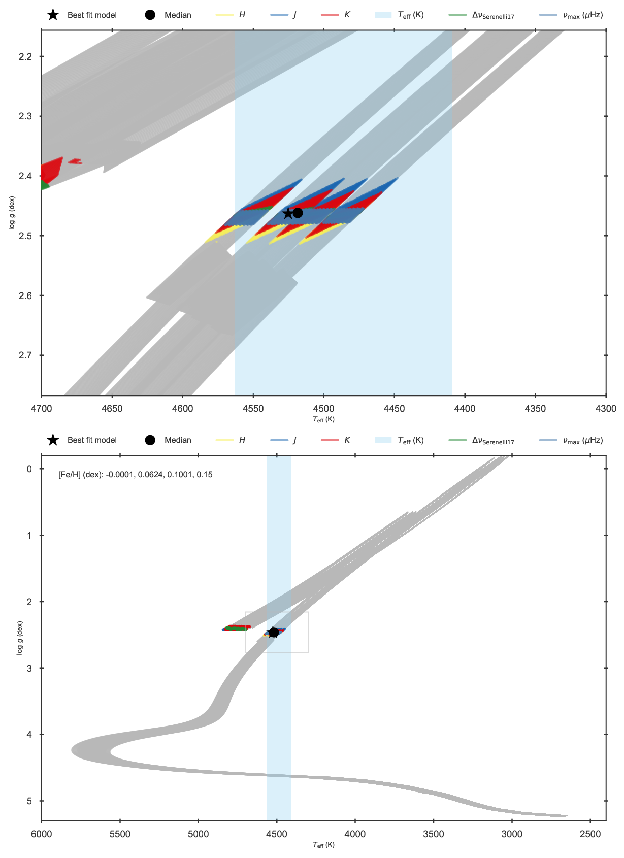
Kiel diagram of the fit to KIC 11129442 including asteroseismology and parallaxes.
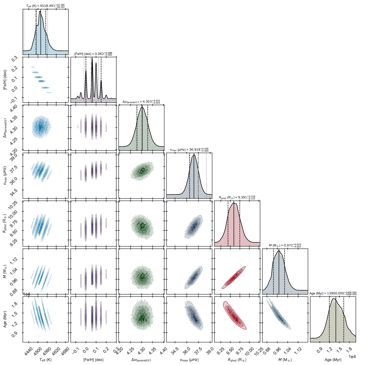
Corner plot of the fit to KIC 11129442 including asteroseismology and parallaxes.
You may have noticed that there is one additional figure to this fit that has not appeared before. This is the corner
plot of the parameters associated to the distance called 11129442_distance_corner.pdf and looks like this:
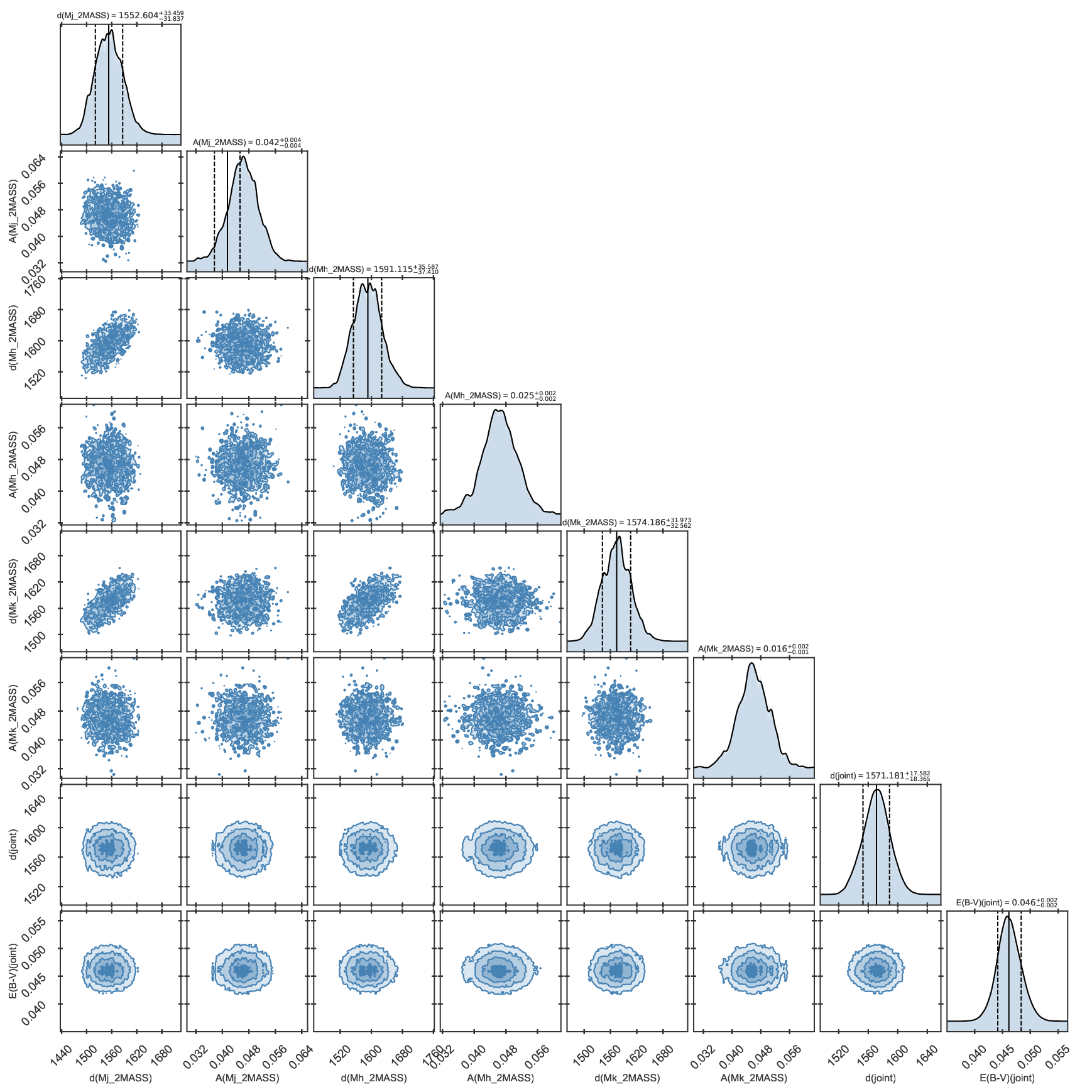
Corner plot of distance properties of the fit to KIC 11129442 including asteroseismology and parallaxes.
In this figure you can inspect the distance distributions and absorptions determined for each magnitude, as well as the
joint distance and extinction distributions. To activate this additional output, the parameter distance must be
included in both define_output["outparams"] and define_plots["cornerplots"]. The example file
BASTA/examples/xmlinput/create_inputfile_parallax.py uses the same parameters in both cases and the plot is
produced.
Estimating distance
One additional feature of BASTA is that distances can be predicted when fitting any quantity. The only requirement is
that in addition to fitparams the user must specify (at least) one apparent magnitude to use in the distance
estimation and provide the target coordinates.
The file BASTA/examples/xmlinput/create_inputfile_distance.py contains the modifications to
create_inputfile.define_input() to produce this fit. The differences with the case of fitting parallax are that
parallax must not be present in fitparams:
# ==================================================================================
# BLOCK 2: Fitting control
# ==================================================================================
define_fit["fitparams"] = ("Teff", "FeH", "dnuSer", "numax")
At least one magnitude must be specified (and of course its observed value and uncertainty should be included in the
ascii file containing the inout data). In this case we will use only the 2MASS J magnitude:
# ------------------------------------------------------------
# BLOCK 2e: Fitting control, distances
# ------------------------------------------------------------
define_fit["filters"] = ("Mj_2MASS")
And finally the parameter distance must be included in the output parameters:
# ==================================================================================
# BLOCK 3: Output control
# ==================================================================================
define_output["outparams"] = ("Teff", "FeH", "dnuSer", "numax", "radPhot", "massfin", "age", "distance")
The distance corner plot including only the J magnitude looks as follows:
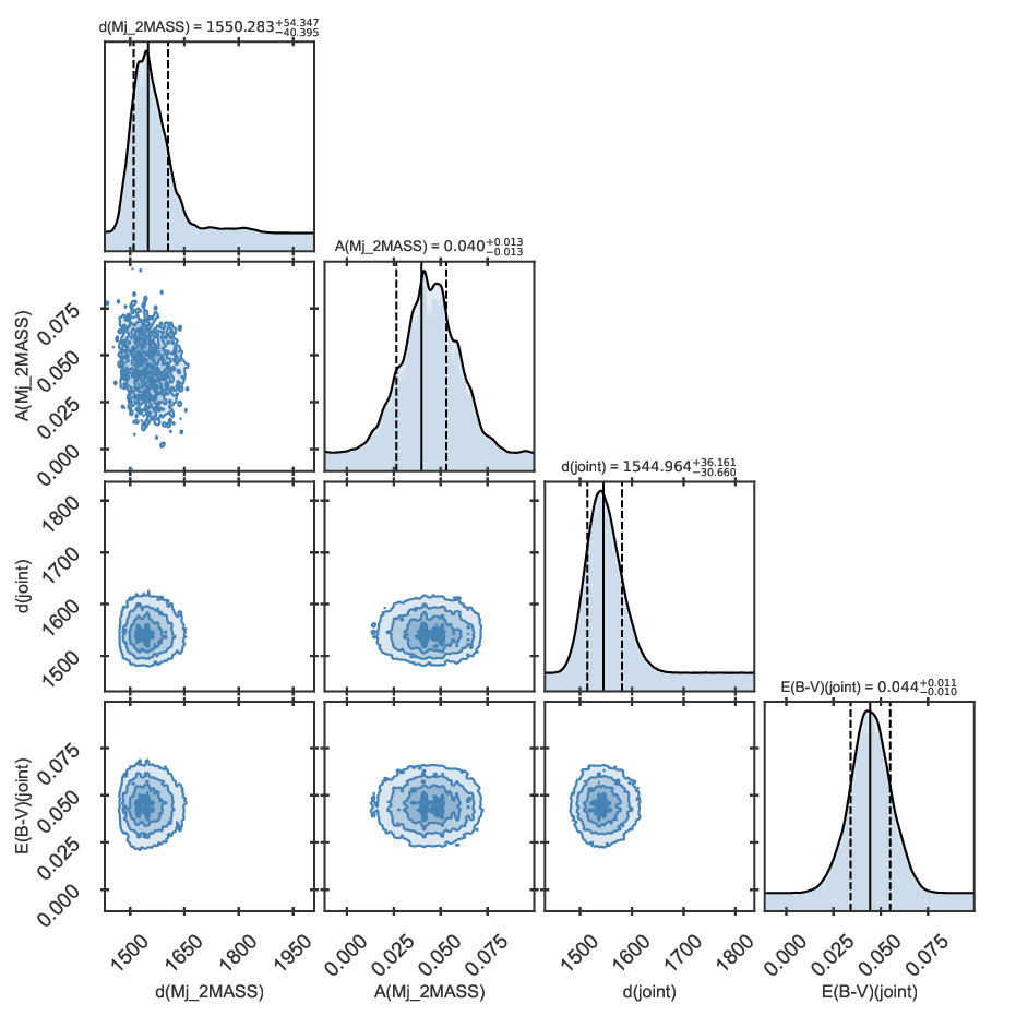
Distance corner plot for KIC 11129442 estimated using asteroseismology, spectroscopy, and one apparent magnitude.
The derived distance is consistent with the value obtained when parallaxes are included.
Fitting evolutionary phase
BASTA offers the possibility of imposing a certain evolutionary phase for a star when this information is known from
e.g., asteroseismic observations. The target KIC 11129442 used in the examples above is clearly an RGB star, and this
information is included in the final column of BASTA/examples/data/Kepler_RGB.ascii as phase. In the
previous fits this information has not been explicitely used, so we show here an example of how to force the star
to be in the red clump phase instead of in the RGB.
The BaSTI isochrones have evolutionary phases assigned following the standarized Key Points given in Table 4 of the Solar scaled paper. Briefly, BASTA names the evolutionary phases as follows:
pre-ms: models [1,99], from Key Point 1 to Key Point 4 (Zero-age main sequence)solar: models [100,489], from Key Point 4 to Key Point 8 (Base of the RGB for low-mass models)rgb: models [490,1289], from Key Point 8 to Key Point 11 (Tip of the RGB)flash: models [1290,1299], from Key Point 11 to Key Point 12 (Start of quiescent core He burning)clump: models [1300,1949], from Key Point 12 to Key Point 18 (Central abundance of He equal to 0.00)agb: models [1950,2100], from Key Point 18 to Key Point 19
In order to see the effects, we recommend you modify the phase column in
BASTA/examples/data/Kepler_RGB.ascii by replacing rgb by clump – or just use the file Kepler_RGB_change-phase-to-RC.ascii where that change has been applied. The file
BASTA/examples/xmlinput/create_inputfile_phase.py contains the settings for an example of this fitting
procedure. The only difference (except for reading the pre-modified data file) is the inclusion of phase in fitparams:
define_fit["fitparams"] = ("Teff", "FeH", "dnuSer", "numax", "phase")
The resulting fit is displayed in the following Kiel diagram where it is clear that the red clump phase has been selected instead of the RGB
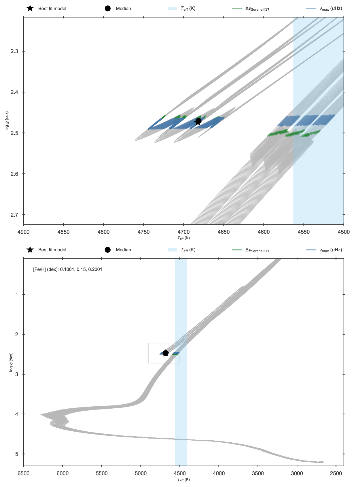
Kiel diagram of the fit to KIC 11129442 forcing the star into the red clump.