Spectroscopy and global asteroseismic parameters

This example describes the fitting of what we call global parameters of the grid, with a specific application to asteroseismology for illustration purposes. As a general recommendation, the user should explore the parameter list for a complete list of available fitting parameters.

Block 2 of create_inputfile.define_input() (in BASTA/examples/create_inputfile.py) defines the fitting parameters. For this example it looks as follows:

# ==================================================================================
# BLOCK 2: Fitting control
# ==================================================================================
define_fit["fitparams"] = ("Teff", "FeH", "dnufit", "numax")

That is, we will fit effective temperature, metallicity [Fe/H], the large frequency separation \(\Delta\nu\), and the frequency of maximum power \(\nu_\mathrm{max}\). Note that the input value of \(\Delta\nu\) is called dnu in block 1 of create_inputfile.define_input(), and the parameter we are fitting here is called dnufit. The reason is that BASTA supports several definitions of \(\Delta\nu\) and it is the user’s decision which one to fit. A description of the various types of \(\Delta\nu\) available is given in Section 4.1.1 of The BASTA paper II, and their corresponding variable names can be found in the parameter list.

The next block to be modified is 2a, where priors to the fit can be selected. We will apply a Salpeter IMF and flat priors in \(T_\mathrm{eff}\) and metallicity, where the likelihoods will be calculated only for models within a certain tolerance from the observed values of each star:

# ------------------------------------------------------------
# BLOCK 2a: Fitting control, priors
# ------------------------------------------------------------
define_fit["priors"] = {"Teff": {"sigmacut": "5"}, "FeH": {"abstol": "0.5"}}
define_fit["priors"] = {**define_fit["priors"], "IMF": "salpeter1955"}

Finally, we define a reference solar model and the assumed solar values:

# ------------------------------------------------------------
# BLOCK 2b: Fitting control, solar scaling
# ------------------------------------------------------------
define_fit["solarmodel"] = True
define_fit["sundnu"] = 135.1
define_fit["sunnumax"] = 3090.0

Note that, in the present example, the solar model is used to scale the grid values of dnufit as described in Section 4.1.1 of The BASTA paper II.

In the folder BASTA/examples/xmlinput/ you can find a file called create_inputfile_global.py that has been prepared following the above instructions to make a fit of the Kepler target 16 Cyg A to the example grid shipped with the code. Simply run the following commands on your terminal:

cd BASTA
source venv/bin/activate
cd examples/xmlinput
python create_inputfile_global.py

You should see the following output printed in your terminal:

**********************************************
*** Generating an XML input file for BASTA ***
**********************************************

Reading user input ...
Done!

Running sanity checks ...
Done!

Creating XML input file 'input_global.xml' ...
Done!


   Summary of the requested BASTA run
----------------------------------------

A total of 1 star(s) will be fitted with {Teff, FeH, dnufit, numax} to the grid 'BASTADIR/grids/Garstec_16CygA.hdf5'.

This will output {Teff, FeH, dnufit, numax, radPhot, massfin, age} to a results file.

Corner plots include {Teff, FeH, dnufit, numax, radPhot, massfin, age} with observational bands on {Teff, FeH, dnufit, numax}.
Kiel diagrams will be made with observational bands on {Teff, FeH, dnufit, numax}.

A restricted flat prior will be applied to: Teff, FeH.
Additionally, a Salpeter1955 IMF will be used as a prior.


!!! To perform the fit, run the command: BASTArun input_global.xml

Once the file is created, run BASTA as explained to perform the fit:

BASTArun input_global.xml

The output of the fit can be found in BASTA/examples/output/global/. It includes a Kiel diagram that should look like the following:

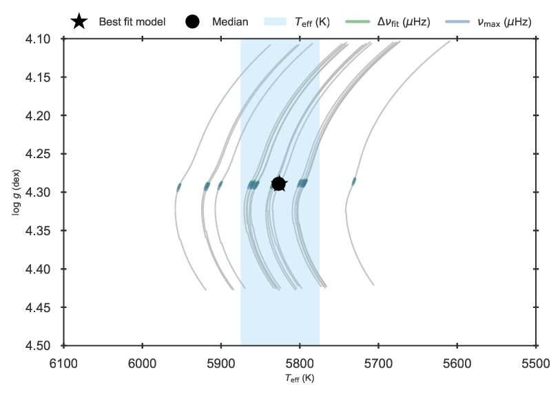
Kiel diagram of the 16 Cyg A fit using global asteroseismic quantities.

This figure is only a visual aid to understand the results, as it depicts the position of the found median and best fit model within the grid. It also highlights in different colours which parts of the grid agree within the uncertainties of the inputted fitparams. Note that the number of tracks plotted are selected to lie within the 16 and 84 percentiles mass and metallicity output of the solution, and are not the only tracks present in the grid nor the only tracks used for the likelihood calculation.

Finally, a corner plot of the parameters included in cornerplots is also part of the output:

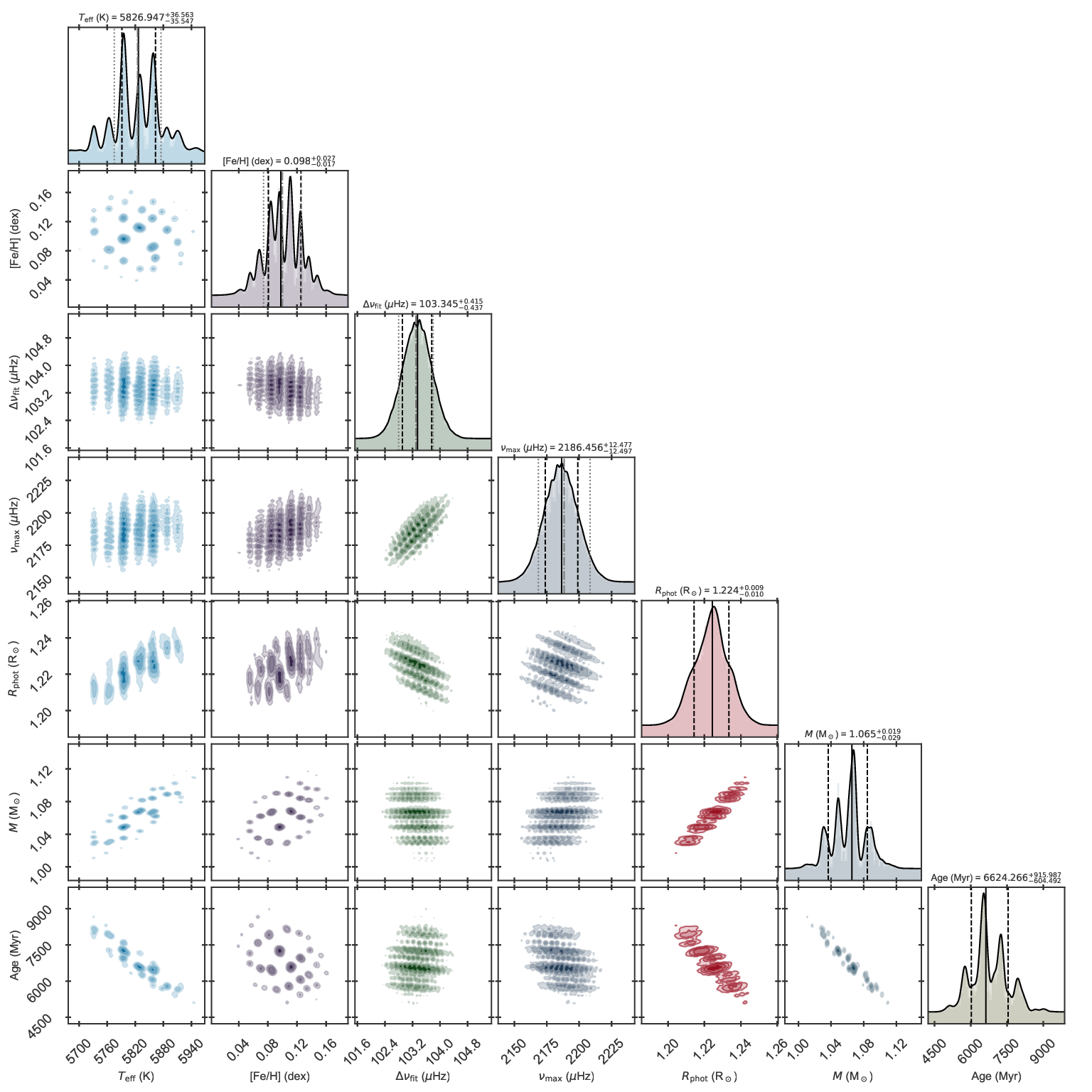
Corner plot of the 16 Cyg A fit using global asteroseismic quantities.

Please note that you might get distributions and numbers with tiny variations compared to what is shown above. This is because BASTA is using using a random sampling scheme to obtain the posterior distibutions. If you want to get exactly the same as in the reference examples, add --seed 42 to BASTArun

Finally it should be noted that the distributions are spiky, which are a reflection of the resolution of the grid (and the small uncertainties on asteroseismic parameters). If you consider this to be an issue for your purposes, don’t forget to check our section on Interpolation of tracks and isochrones.

Congratulations! You just completed your first fit using BASTA. Easy-peasy, right?